Three Pin

Depending on how much room you have on your hard drive you should either copy the entire web_tele folder from the C/D to you hard drive or copy the much smaller surf_prog folder to your hard drive.  Then change the attribute on all the surf.html files from read only so you can edit them with Notepad or other text file editor.

Editing the HTML file makes sense because many things do not change often.  Your mirror diameter and whether or not the light source on your tester moves are examples.

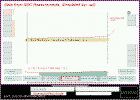
In the picture of a surf.html file at right I highlight the PARAM(s) that I changed for 'Three pin'.

• Mirror diameter and radius of curvature.

• The PARAM for center obstruction diameter was set to a negative value which will change its function to 'L' value.

• The units for the knife edge data entrees were all changed to units of millimeter and set to zero.

• Light source moves was set to "false".

• Auto recalc was set to "TRUE" in capital letters.  This causes the program to bypass the wedge display on start up and also display the plot board without the overlay picture.   'w' on the keyboard will still activate the wedge display if needed.  Esc will bring up the background legends for the data entry buttons if needed.

• Marker pins was edited to have only three pins active on startup.  Pin number zero is reserved so we assign the inner data entry, 15 percent, to pin one then 70 percent to pin two, then 95 percent to pin 3.  The remaining five pins will remain set to less than zero percent which will define them as undefined.

Start the program by clicking on:  Three Pin

Press Esc to bring up the data entry background legend.

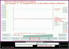
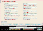Looking at page one we see the Applet read the PARAM(s) for mirror diameter and radius of curvature and calculated an F# of 7.8.  

Using the -7.25 inch 'tube center' to 'primary focal plane'  the program calculated a diagonal size of about 1 1/2 inches.

If we have a 10 millimeter eyepiece that would give a magnification of about 160x.

The file name which was entered displays at the bottom left.
This file name entry is not used unless you use the  bmp_to_txt  program.
Anything could be entered here.

<!-- "My Mirror" -->
<PARAM NAME=disp_legend Value="surf_three_pin.html " 

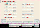Looking at page two we see the data entrees for knife edge measurements in millimeters.

The units for the  R' minus R_o box are also in millimeters as are the units for 'Caustic' on page one.  These units were initialized from the zone_units PARAM in the .html file.  The R' minus R_o box is showing the value of r_sq over 2R at 100 percent.

Presume we get the following data from our test 'engine' ( that has the fixed light source ).

Percent	Reading in mm
15	0.85
70	1.60
95	2.90

So I enter the readings and press the 'Clear' key once.  And there is plotted the curv_fit_to_data[] array which has been set to fit the entered data points.

Press 'Show Screen' ( lower right corner ) to turn off the data entry boxes.

Press the second button on the left side of the plot board. Plot board control will attempt to display:

"  ROC Measurements Curve minus R' - Ro = rsq/2R, parabola.  ".  However the request will not succeed because the formu_starward_metric[] array has not been filled and is null.  Since the auto_recalc PARAM is set to true the program will press the 'Start Plot' button and then return.  As the formu_starward_metric[] is filled the progress will be plotted.  Press the second button on the left again and this time the request succeeds.   curv_fit_to_data[] and formu_starward_metric[] are plotted as 'ghost' and the difference in color.

Press the top left button on the plot board.

Press the 'Set pin [o]' button.  The set_data_for_marker_pin_0_to_the_curve()  method sets the radius of the reserved pin number zero to a percent zone such that half the mirror surface is inside of that radius and half of the mirror surface is outside that radius.  That radius would normally be the 70.7 percent zone, however on this mirror the center will be blocked by the shadow of the diagonal so pin zero is set to the 71.8 percent zone.

The method set_data_for_marker_pin_0_to_the_curve()  may return at this point or proceed to set pins at  0 percent and 104 percent.  Whether or not pins are set at 0 and 104 depends on whether there were already a pins at those radii and also whether there are deactivated pins to use for this purpose.  The method tries to set the pin at 104 percent first and if that succeeds tries to set the pin at 0 percent.

To find how far the method succeeded press the 'Show Marker' button.  And we see that all three pins were set.

Press the 'Show Plot' button.  It seems that pin seven at the mirror center was set a bit low because when we did the Foucault test the mirror center did not seem to be low.

So I reset pin seven from  -.03228 mm to  .8 mm.  Now the curv_fit_to_data[] array seems to have a curve that represents this mirror.   Note that the previous plot is still visible temporarily in a lighter shade of the same color. 

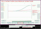Next press the third button on the left.  We would see the surface transform of the 'starward' array if the surface plot scale were set to about 5000 Lwave.  ( The tranform of curve_to_fit_data[] is the data__surface_metric[] array. )
With the surface scale at .5 Lwave you see plotted data__surface_metric[]  minus parabo_sag_metric[].  In cyan is plotted the wave front error.  Note the group of four buttons on the lower right of the plot board.  There is no black 'alert line' for the second button.  The second button was selected as the program started.  It is the parabolic surface array parabo_sag_metric[].  The absence of the alert bar means that the p_transform_correction_array[] has been filled and is ready for use by the starward_to_surface_transform() method.

Next we press the 'Zero Data' button and data__surface_metric[] and parabo_sag_metric[] are zeroed at pin number zero ( at 71.8 percent ).  Pin number zero had the focus when the 'Zero Data' button was pressed.  If a different pin had the focus the arrays would have been zeroed at the different pin's radius.  Note the blue alert lines. The blue alert lines show which arrays have been zeroed at a new  r_x.

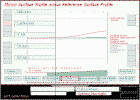
Next press the fourth button on the left.  The plot_surface_minus_reference_surface() method now plots data__surface_metric[]  minus parabo_sag_metric[] times a weighting factor for mirror surface area.   By weighting for the area of mirror surface represented at each percent zone a more realistic representation of mirror performance is presented at the RMS display at the right of the plot board .  Using this setting the mirror center looks perfect but then the mirror center has no surface area.     Operation and options for circumference weighting. 

Next press the fifth button on the left.  The plot_surface_minus_reference_surface() method now weights the plot with wave front error.  If one point on the mirror were 1/4 wave in error from the rest of the mirror the light from that point would be 180 degrees out of phase with the light from the remainder of the mirror thereby canceling part of the signal.  If the mirror surface error decreases from 1/8 wave surface error the effect on the wave front decreases rapidly.

In the final frame of picture six we have pressed the  o key on the keyboard. This bypassed 3/2r weighting for surface area.  Pressing the o key also changed the plot color thereby repainting the image and in a different plot color.

Every time a surface is plotted by plot_surface_minus_reference_surface() the RMS value is calculated and posted to the right of the plot.  The RMS calculation is explained by R. F. Royce on his web page.  As explained on the web page the RMS value or any measure of a mirror is only of use if it means the same thing to everyone.  And as you can see the RMS value calculated by the Surf program depends on the reference point on the mirror as well as whether the surface weighting and wave front weighting are used.

Using a Mirror Surface Formula as a Mirror Surface Reference

In the 'Three Pin' example above it was expected that the mirror center would be high but all the error showed up at the mirror edge.  I set the percent data entry box to 15, 70 and 95  to view the formula 'R'- Ro at those zones.   70 and 95 percent measurements seemed to be close but the 15 percent measurement was high.  But then the true answer depends on the radius of the parabola that we use for the reference.  So instead of just using a reference parabola with the radius of the mirror center I made a series of plots and slowly shortened the radius of the reference parabola.  The .html file for this example is: surf_three-pin_data-entered.html.
In  surf_three-pin_data-entered.html  the  PARAMs  were prepared by using the same data as in three-pin.html .   After all the entries were made in three-pin.html and the starward data zeroed at the mirror center I copied the values, now having been offset, out of the data entry boxes and entered the values into three-pin_data-entered.html.  Now I can start the program with the same mirror figure without re-calculating values for 0 percent and 104 percent each time.

The animated .gif graphic at right shows the result.  The screen was captured with PrintKey and the editing done with PBrush and the layering with LView.

The result shows that the RMS value is better when using a reference parabola .0125 inch shorter in radius than 125 inch.  And after weighting for surface area and wave front cancellation the best reference is .0150 inch shorter than 125 inch.

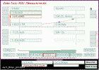The animated .gif at right shows a step by step procedure used to prepare one frame of the .gif.

First we need the formula_as_a_surface_metric[] array ( the reference array ) filled with entries for a shorter radius parabola.  Formula 3 in the .html file has been edited to:

<PARAM NAME=function03 Value=" ( r * r ) / ( 2 * R ) ">  Which is the formula for a parabolic surface.

Start the Applet and change the ROC data entry to 124.9975 inch.  Frame B in the animation.
Changing the ROC or the mirror diameter nulls several of the arrays as indicated by the alert lines.

Frame C:  Select function 3, the formula for a parabolic surface.

Frame D:  Click 'Start Plot' to fill the formu_starward_metric[] array.  
                    As the array is filled a plot is made.

Frame E:  Right click on the button PBRB4, 'Use Formula 3 as a Mirror Surface Reference'.  The alert line changes to green as the formula_as_a_surface_metric[] array is instantiated and the contents of the formu_starward_metric[] array is copied into it.

Frame F:  Reset the mirror ROC back to 125 inches.  This nulls several arrays but does not have any effect on  formula_as_a_reference_starward_metric[] ( not used in this example ) or formula_as_a_surface_metric[] which we just prepared for our surface reference.

Frame G: We clicked the clear button twice.  Later I found that not clearing Surf at this point still gives the same calculation result.  Had I held down the  x key  during clear the formula_as_a_surface_metric[] array just loaded would have been lost.

Frame H:  Click on the 'Show Screen' button on the bottom right corner to turn off the data entry buttons.

Frame I:  Click on the top left button to refresh the 'Data from ROC Measurements' display.

Frame J:  Click on the 'Set Pin[o]' button.  Pin number zero is set to 71.8 percent as before and its data value is given the data value of the curve_to_fit_data[] at that radius.
Next the method tries to set a pin at 104 percent but finds there is already a pin at that location.  So the method displays a note on the status line and rings the bell and returns.

Frame K:  Left click on the 'Use Formula 3 as a Mirror Surface Reference' button.
Had the surface array not been loaded, Frame E, a note would have been displayed.

Frame L:  Click on button L3, 'Mirror Surface Profile Minus Reference Surface Profile'.

Frame M:  Click on 'Zero Data'.  Since pin number zero had the focus data__surface_metric[] and formula_as_a_surface_metric[] are zeroed at 71.8 percent.  Blue alert lines are displayed.

Frame N:  Click on button L3 to refresh the display.
Made a screen capture using PrintKey for the upper part of the animated .gif.

FrameO:  Click on button L5 to get MSP - RSP weighed for mirror surface area and phase.
Made a screen capture using PrintKey for the lower part of the animated .gif.

 

'Quantify' a turned Edge

The file for this example is surf_ronchi-alternate.html.
Formula two in this file is the same as formula two in ronchi-alternate.html.

Frame B:  Select formula two.

Frame C: 'Start Plot' then select formula as a data source by pressing the second button of the data source selector buttons.  ( Top right buttons )

Frame D: With the mouse hovering over the top left button the legend shows:  'Data from ROC Measurements, Simulated by: null'.   Note that making the selection at Frame C did not make the selected formula data available.  
It is possible to have one starward formula in curv_fit_to_data[] when formu_starward_metric[] has been changed to a different formula.

Frame E:  Next press the top left button and the legend reads 'Data from ROC Measurements, Simulated by: R' - Ro formula f2(r,R).   When the formula is selected as a 'starward' source then every time you press the top left button curv_fit_to_data[] will be overwritten by formu_starward_metric[].

Frame F: Pressing the third button on the left performs the transform and we can read the wave front error.

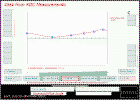surf_ronchi-alternate.html provides a good opportunity to demonstrate an error I made several times while testing Surf.  It may not be obvious but when one uses 'Set Pin[o]'  the data values for the pin that may be set at 104 percent and the pin that may be set at  0 percent comes from an extrapolation of the data value of pin number zero at 71.5 percent in this case. The extrapolation is done using whatever formula happens to be loaded in formu_starward_metric[].  In the frames at right I load formu_starward_metric[] with formula R' - Ro formula f1(r,R) which is definitely not the formula for the knife edge measurements from a parabola.  And you can see the data for pins at 0 and 104 percent were not set as I had expected.
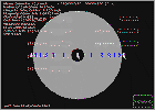To recover from this press the 'Zone Marker' button to obtain the screen at right then click on the pin at 0 percent and the pin at 104 percent. This will deactivate them again.   Then turn on the plot board and select the correct formula then press 'Start Plot' then try 'Set Pin[o]' again.  If you try 'Set Pin[o]' again without deactivating the pins at 0 and 104 percent then 'Set Pin[o]' will give explanations in the status bar as to why the request failed.  To set pin zero and bypass the procedure for putting a pin at 104 percent and 0 percent hold the space bar down when you press 'Set Pin[o]'.
To properly display a mirror surface for a mirror which is only partially parabolized one could select a formula which sets pins at 104 percent and 0 percent correctly.  Better than that is to obtain information about the mirror using Ronchi and Foucault tests and manually re-adjust the data for pins at 104 and 0 percent.  If one suspects a turned down edge, for example, one could set data for pin 104 slightly high to produce a mirror surface with a turned down edge.  If the mirror is only partly parabolized and data for the pin at 0 percent has been set by an extrapolation of pin# zero ( at 70 percent ) then the pin at zero percent will be too low.  Unless your mirror actually has a low zone in the center then the data for the pin at zero percent will need to be adjusted manually to get an accurate surface representation after the transform.  Refer to the 20 inch mirror example.

 

Precision Calibration of the Transformer Method for Non Parabolic Mirror Plots.
Review of Surf Program Accuracy.

The file for this example is surf_conic.html.   All the examples above have used the p_transform_correction_array[] for precision calibration of the output of the of the 'starward' to surface transformer method.   The s_transform_correction_array[] is used to calibrate the output of the transformer to be precisely correct for a sphere.  And the x_transform_correction_array[] can be used to calibrate the transformer for use with surface reference selections 1 and 4.  Thus if one were making a very precise ellipse, for example,  it would be possible to custom calibrate x_transform_correction_array[].

The two legends above are visible on the plot board when hovering over surface reference selector button one and button four. ( PBRB1 and PBRB4 )

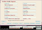At right is a picture showing the mirror properties for this example.  If you open surf_ronchi-conic.html using notepad you will see the PARAM(s) below.   
function01 is a starward formula for conic curves.  By changing B, the conic constant, in function01 it is possible to custom select a conic.
function02 is a surface formula produced by using the 'quadratic equation' on a precursor version of the formula, fuction01. 
function03 is the starward formula for a parabola derived using trigonometry.

<PARAM NAME=function01 Value=" ( R * ( ( 1 - B * r ^ 2 / R ^ 2 )^1.5 ) - R ) / 3 "> 

<PARAM NAME=function02 Value=" ((-2 * R)-SQR(((R*2)^2) - 4*r*r * ( 1 + B )))/2 * (1+B)">

<PARAM NAME=function03 Value=" S + ( TAN( .5 * ( IVT( r / (( R / 2 ) - S ) ) ) ) ) ">

<PARAM NAME=constant_A Value="-.666 "

The data values for the zone pins were calculated by plotting R'-Ro formula 1.  Then I set the percent data entry to each zone and copied off the R'-Ro values for later entry into the surf_conic.html  PARAM(s).   B in the formula is the 'conic constant' which is set in the PARAM(s) to -.666 .  ( The initialization of constant_A also initializes constant_B with the same value. )

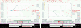The two pictures at right show the resulting transform referenced to a parabola and then a spherical surface reference.  In the picture showing the parabolic surface reference you can see the red alert bar to the right of the spherical selector button. The red alert bar indicates the s_transform_correction_array[] has not yet been calibrated.  The amber alert bars to the right of 1 and 4 button show they would use p_transform_correction_array[].

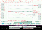The picture at right shows I have used the transform of the starward formula as a surface reference.  The plot shows the mirror edge is about .003 LWave low. The wave length in this case was set to 300 nm in the PARAM(s).  Did this surface error come from the curve_fit_to_entered_data_points() method or from the starward_to_surface_transform() method?

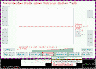My first idea is to substitute formu_starward_metric[] data in place of curv_fit_to_data[] data which I did in the animation at right.  This does indeed bypass curve_fit_to_entered_data_points() but now the accuracy of starward_to_surface_transform() seems unbelievably good as shown on the last frame of the animation.  Unfortunately this is not really a test of starward_to_surface_transform().  All it tells me is that starward_to_surface_transform() did exactly the same thing when it filled the unknown's surface array as it did when it filled the reference surface array.

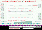Next I select button 2 on the left which subtracts the starward reference from the curve fit to the entered data.  Subtracting formu_starward_metric[]  from  curv_fit_to_data[]  indicates the error present before the transform.

The curve_fit_to_entered_data_points() method was mainly tested on a 10 inch F5 parabolic mirror.  Then a bit of "tuning" was done to improve the performance at F4.  For mirrors 'faster' than F4 expect increasing errors.  For mirrors with ROC's greater than F4 the accuracy is better than for F4.  Also expect increasing error as we go from ellipse to parabola to hyperbola which increases the non linearity of the curve that  curve_fit_to_entered_data_points() must interpret.   The curve is also more curved with a tester with a stationary light source.

Now to try to find the error in the transformer method caused by using p_transform_correction_array[]  on a curve that is not a parabola.

To calibrate x_transform_correction_array[]  the user must find a formula that describes the starward data and another formula that describes the surface data then use the fill_transform_correction_array() method to fill the x_transform_correction_array[].

fill_transform_correction_array() uses the formula_as_a_reference_starward_metric[] array as the starward calibration reference and the formula_as_a_surface_metric[] array as the surface reference.  We have filled formula_as_a_surface_metric[]  before by a right mouse click of button 4 of the surface reference selectors.  To fill formula_as_a_reference_starward_metric[] we use a right mouse click on button 1 of the surface reference selectors.  When formula_as_a_reference_starward_metric[] has been filled there will be a green alert bar to the right of button 1.  ( Note that the green alert bar is drawn when formula_as_a_reference_starward_metric[] is filled and if you use 'Clear' later formula_as_a_reference_starward_metric[] and formula_as_a_surface_metric[] will still be there even though the green alert bars are gone.   If you press the x key during 'Clear' then  formula_as_a_reference_starward_metric[] and formula_as_a_surface_metric[] will be nulled. )

When the fill_transform_correction_array() method is called and finds that neither formula_as_a_reference_starward_metric[] nor formula_as_a_surface_metric[] are null it will display the user prompt:

You must either hit the  t key or the  f key on the keyboard.  If you hit the  f  key the program will continue to use p_transform_correction_array[] as the default correction array even though both formulas are not null.  If you hit the  t  key the x_transform_correction_array[] will be filled and used as first choice for button 1 and button 4 of the surface reference source selector buttons.   If starward formula 1, in this case, does not correspond to surface formula 2 and you still answer  't'  then the  starward_to_surface_transform() method will produce unbelievably strange results.

The thumbnail at right takes you to a two frame gif that shows a result of using the p_transform_correction_array[] and then the x_transform_correction_array[] on a transform of
" ( R * ( ( 1 - B * r ^ 2 / R ^ 2 )^1.5 ) - R ) / 3 ".  
The surface reference is: formula_as_a_surface_metric[], 
"((-2 * R)-SQR(((R*2)^2) - 4*r*r * ( 1 + B )))/2 * (1+B) "  which was selected by a left click on button 4R.  Using the p_transform_correction_array[] indicates about .007 of a wave error.  Using x_transform_correction_array[] shows no error which is not surprising since x_transform_correction_array[] was calibrated using
" ( R * ( ( 1 - B * r ^ 2 / R ^ 2 )^1.5 ) - R ) / 3 " and  
"((-2 * R)-SQR(((R*2)^2) - 4*r*r * ( 1 + B )))/2 * (1+B) ".

Note that  "((-2 * R)-SQR(((R*2)^2) - 4*r*r * ( 1 + B )))/2 * (1+B) "  is meaningless if conic constant B is -1.  In the animation at right we set the conic constant to -1.00001 and look at the surface error.  With the scale magnification set large we see there is a strange type of noise. I suspect the noise is cause by the calculations being near the limit of precision of the double precision data type used in the computers calculations.

In the next image for surf_conic.html the program is showing the error produced by the data pins that were set by copying R'-Ro values into the PARAMs.  The two frame gif shows the error at 300 nm wave length and 600 nm wave length.  Note, to get the nm display turn the 'wedge display' on then off with the  w key.

In the final image for surf_conic.html we test the effect on program accuracy ( in wave lengths ) of doubling mirror radius and diameter.  We forgot to change secondary diameter.  The users data is overwritten with a conic of -.999 to generate an error in reference to the default parabolic surface reference.

 

 

Simulation of Atmospheric Turbulence using Random Numbers

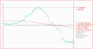The file for this example is surf_RAND.html.   In this example the formula:
"((r*r)/(2*R)) * (1-(3*.00003*W*r))+(B*RANQ)"
is used to fill the 'starward array'.   The starward array overwrites curv_fit_to_data[] then curv_fit_to_data[] is transformed to a mirror surface and compared to the reference parabola.

The B parameter is adjusted to produce a wave front distortion to suit the user.  In this case I first recorded a series with B set at 2.  Then a second series with B set at 8.  The upper frame in the animation is presumed to be excellent 'seeing' at sea level in the San Francisco area.  The lower frame is presumed to be typical seeing.  Excellent seeing would show steady diffraction rings now and then with the eyepiece slightly de focused.  Typical seeing would be available 95 percent of the time if there is no fog.  In the daytime or with the telescope mirror not at ambient air temperature the seeing would be expected to be five or ten times worse than typical.

One possible interpretation of the mirror surface is that it represents the excursions of an adaptive optic mirror.   Note that conic curves such as the parabola are the only curves that will allow all the light to arrive at the focal point in phase.  Some abberations would allow all the light to cross the focal plane in phase or have all the rays directed to the focal point but out of phase.  It is my understanding that having the rays out of phase reduces the amplitude from peak value to what is called RMS amplitude.  The power in the wave is equal to the square of the amplitude.

In the formula:
"((r*r)/(2*R)) * (1-(3*.00003*W*r))+(B*RANQ)"
the r*r/2R term is the familiar starward formula for a parabola.  RANQ is derived from RAND.  ( See view_sou.htm for notes on RANQ and W. )  RAND produces random numbers between 0 and 1. The random numbers don't look like turbulence or 'dog biscuit'.  So .5 is subtracted to make the numbers symmetric as to zero.  A running RMS calculation of six random numbers reduces the high frequency component of the random numbers.  Due to squaring the RMS value is always positive so if the average of the same six random numbers is less than zero the sign of the RANQ output is set negative ( after the square root has been taken ).   
'W' is used as a 'negative feedback' term.  ( Negative feed back as in a 'servo system'.  )   In order for 'W' to be functional, formula_as_a_reference_starward_metric[] array must be loaded with r*r/2R formula by a right mouse click on reference surface button one as shown in the animation below.  Note that formula_as_a_reference_starward_metric[] need only be loaded before the first frame of a sequence of turbulence frames.

Refer to the animation at right.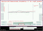

Frame B: Fill formu_starward_metric[] with r*r/2R.

Frame C and D: Right mouse click to copy formu_starward_metric[] into formula_as_a_reference_starward_metric[]

Frame E: Select "((r*r)/(2*R)) * (1-(3*.00003*W*r))+(B*RANQ)"

Frame F: Set 'Starward Reference Source'  to formu_starward_metric[] and
Fill formu_starward_metric[] with "((r*r)/(2*R)) * (1-(3*.00003*W*r))+(B*RANQ)"
Note that in addition to the normal plot of  formu_starward_metric[] the value of 'W' is also plotted ( in blue ).  If 'W' is used in the formula it will always be plotted.

Frame G: Hold the space bar down and click 'Set Pin[o]

Frame H: Overwrite curv_fit_to_data[] with formu_starward_metric[]. ( L1 button )

Frame I:  Display the transform.

Frame J: Zero the curve at 72.1 percent zone.

Frame K: re-display.

 

 

Prepare a table of Caustic X and Y  Values for the test described in ATM Book Three

The file for this example is surf_caustic.html.   In this example the light source does not move, same as in the example in ATM Book Three.

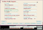Refer to the animation at right.

Frame A:  Click the mouse on the Applet field to obtain the keyboard focus.  Press the  Esc  key.

Frame B:  Change to page one.

Frame C:  Enter the desired percent zone into the percent data entry. 

Frame D:  Press the  c  key to activate the caustic display.  Enter the X caustic value in your table.

Frame E:  Press the   c  key and enter the Y caustic value in your table.

Frame F and G   Continue until the zone are all entered.

Note the caustic values given use the formulas in the ATM book.  The displayed value does not depend on the selected R'-Ro formula as does the R'-Ro values displayed in the same location when page 2 is selected.

zone	radius	percent	Y	X
0	0	0	.000	.000
1	1.1	18.3	.02989	.00036
2	2.2	36.7	.12022	.00292
3	3.3	55	.27	.00982
4	4.4	73.3	.47956	.02324
5	5.5	91.7	.75055	.0455

An empty caustic table.

 

 

What does a parabolic curve look like.

Its hard to see the difference between a sphere and a parabola on a long focus mirror.  If we make the radius of curvature very short the difference is easy to see.  The file for this example is surf_caustic.html.

The upper plot which is 'curve to fit data' is irrelevant in this example.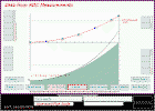
Refreshing the lower plot by changing the 'R'-Ro' selection will bypass the normal clip which is at the bottom of the scaled portion of the plot board. Refer to the animated picture at right.
Selecting the wedge display with the  w  key and selecting plot board button L1 or L2 will also bypass the normal clip.

On my computer monitor which is about 17 inches a 12.6 inch mirror will plot 1 to 1 scale in the lower plot.   That with monitor display properties set at 800 x 600.  The radius of a mirror is always 400 pixels on the plot board. When using a custom formula the radius of the mirror is 200 pixels.  The reason for this is that the formula parser derived from the Ronchi/Foucault program which used 200 pixels for mirror radius.

 

Program/User interface Problems

You may have noticed that when you clear the program by clicking on the 'Clear' button twice the screen looks unusually clear.  The program calls the clear method when it first starts but then draws the screen as if the PBL1 button had been pressed.   So you never saw the screen completely cleared until the clear method was called without redrawing something.

If you use the browser ''Back' button on some browsers and then the 'Forward' button the program will keep the state of the Java code in your computer's memory the same as it was and re-start the 'Surf' Applet by calling its init() method.  I have tried to make the 'Surf' program restart as it would if initialized the first time but there seem to be some differences.  So press the 'Clear' button twice if there is some seemingly inappropriate display after re initializing.
To avoid this re-initializing problem it is possible to start a new instance of the browser by clicking on the browser's screen area to actuate its keys then press Ctrl  n  to start a new instance of the browser in the computer's memory.  Then you can view the instructions in the second browser without re initializing the running 'Surf' program.
A similar 'out of sequence' condition may occur after some unusual combination of clicks on buttons.  So try the 'Clear' button and most likely the program will return to normal.

When using the formula as a surface reference PBRB4 you will need to left re-click on that button after some program sequences because the program defaults back to the parabolic surface reference PBRB2 after some program sequences.

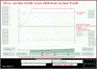The thumbnail at right links to an animation that show the same surface display at two different vertical scales.  In this case the surface reference had a slightly different ROC which shows as a surface error in the unknown plot minus reference surface plot. ( brown line).  When we change the scale to 5000 waves we see the actual unknown mirror surface plotted in gray and the reference surface from the formula as a surface plotted in amber.

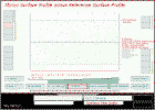In the thumbnail at right we have a reference surface formula so different from a parabola that the difference shows up in the amber reference surface formula's plot when the scale is set to 5000 waves.  In this case the cause was that the conic constant in the surface reference formula was set to -3 instead if the usual -1.
Setting the display scale to 5000 waves ( or some such large value ) is also useful when looking for errors in the setup of the x_transform_correction_array[].
You will need to hold the   x   key down while using 'Clear' after x_transform_correction array problems.  That since the starward and surface reference arrays may contain the wrong curve(s).
Another reason for an unexpected difference between gray mirror data curve and the amber reference curve is that if the curves have been zeroed at a data point.  When this is done with, for example, the gray unknown curve and the amber parabolic curve then both of the entire array's values are shifted up or down on the plot board.  Now if we select the spherical reference for the amber reference curve we would expect that the change in the curve would be only the difference between a sphere and a parabola but because the gray curve was shifted previously and the spherical array for the amber curve presumably has not been shifted the result is a very large error.

 

In surf_Dianna.html the person getting the knife edge readings didn't bother to get a reading at the 31.6 percent zone.  My first thought was to set that data point to zero, but that gives an obviously incorrect result.  The second idea was to just set that data point to a value that "looks right",  but since I didn't actually look at the persons mirror that's not too good an idea either.

The final idea was to just not put a data point at 31.6 and let the curve_fit_to_entered_data_points() method handle the job.  To do this I changed the PARAMS in the .html file using Notepad.

 

 

 

 

Return to the instructions page.