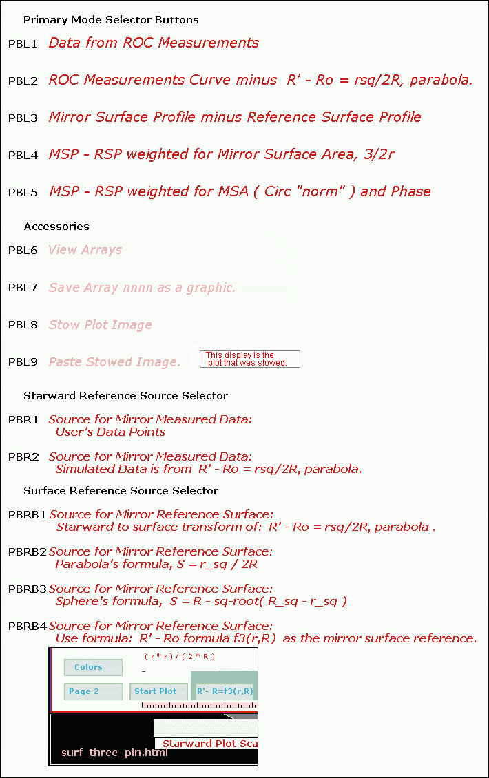
Plot Board Buttons
Legend will always display the 'Primary
Mode Selector Buttons' state
unless the mouse cursor is on some other button.

| Primary Mode selector Buttons | |
| PBL1 | If PBR1 is selected displays curve to fit data.
If PBR2 is selected displays the R'-Ro output of the formula parser. PBL1 will always plot the previous plot in a lighter shade. |
| PBL2 | Always displays 'curve to fit data' minus R'-Ro output of
the formula parser. If the 'Color' has been changed PBL2 will plot the previous plot in a lighter shade. |
| PBL3 | Surface plot
Draws the unknown surface and marker pins. |
| PBL4 | Surface plot
Draws the unknown surface and marker pins. |
| PBL5 | Surface plot
Draws the unknown surface and marker pins. |
| Accessories | |
| PBL6 | View Arrays, refer to graphic. Allows the user to obtain values from the following arrays: 1 'Curve to fit data'. 7 The result of subtracting one of the above arrays from
another of the above arrays. 8 An estimate of how a certain change in starward will affect
surface. |
| PBL7 | Using the 'Save Array' selection it is possible to save (
to disk ) one of the
400 element arrays of mirror surface or starward data. The array to
be saved is selected from the 'View Arrays' page. See
PBL6. Instructions for using 'Save Array'. |
| PBL8 | Copies the image of the plot board to an off screen image in memory ( not disk ). |
| PBL9 | Displays the image copied by PBL8 to the plot board. Displays a note to the user since the display may not correspond with the 'Primary Mode selector Buttons' selection. |
| Starward Reference Source Selector | |
| PBR1 | Default, PBL1, unknown curve. Use 'Curve
to fit data' which is derived from the users data measurements. |
| PBR2 | PBL1 will overwrite 'Curve to fit data' when PBL1 is
pressed. PBL1 is overwritten with R'-Ro array, formu_starward_metric[]. |
| Surface Reference Source Selector Hovering the mouse cursor over these buttons will call the 'fill transform correction array' method if the associated transform correction array has not already been calibrated. Note: Fill transform correction array method is locked out when a curve has been zeroed at a data pin. |
|
| PBRB1 | User must provide a starward formula which will be
transformed to use as a surface reference. Draws the transform of users curve on the plot board and the cross section. Next time a 'Primary Mode selector Button' is pressed transform of users formula will be used as the surface reference. Right mouse click loads formula_as_a_reference_starward_metric[]. Ref1 Ref2 |
| PBRB2 | Draws a parabolic curve on the plot board and the cross
section. Next time a 'Primary Mode selector Button' is pressed formula for a parabola will be used as the surface reference. |
| PBRB3 | Draws a spherical curve on the plot board and the cross
section. Next time a 'Primary Mode selector Button' is pressed formula for a sphere will be used as the surface reference. |
| PBRB4 | User must provide a surface formula to use as a surface
reference. Draws the users curve on the plot board and the cross section. Next time a 'Primary Mode selector Button' is pressed users formula will be used as the surface reference. Right mouse click loads formula_as_a_surface_metric[]. Ref1 Ref2 |
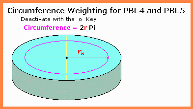 |
'o' toggles (on/off) a normalized
'O' toggles (on/off) weighting by zone
|
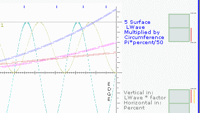 |
'Wedge
Display' activated, 'w'
key. Picture at left shows the three possible setting for circumference weighting of PBL4. Activation of the 'o' or 'O' key also causes plot color to change. |
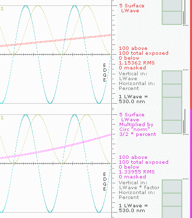 |
'Wedge
Display' activated, 'w'
key. Picture at left explains the reason for the 3/2 factor of the "norm" circumference weighting. If the error is 0 at the mirror center and increases straight line ( linearly ) to the edge the area under the curve will be the same with 3/2r factor on or off. Note: Secondary mirror diameter must be set to zero for this demonstration. |
Display Arrays, PBL6
|
Example, subtract a spherical array from a parabolic array and display the result in inches.
To cancel an undesired amber button hover the mouse over Esc |
Notes on the Wedge Display, Conic Display and Cross Section.
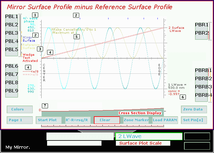
| Wedge Display When the wedge display is activated by pressing the w key on the keyboard then method 'plot surface minus reference surface' will not plot unknown surface minus reference surface. A wedge array will be substituted in place of the normal difference array plot. The wedge vertex is at the mirror center and the wedge is two waves deep at the mirror edge. |
|||||||||||
| 1 |
|
||||||||||
| 2 | The mirror surface plot which is the transform of
'curve to fit data' is plotted in gray. The pins are plotted in blue. If a pin has the focus it is plotted in a different shade of blue. To see this plot it may be necessary to increase the number in the 'Surface Plot Scale' data entry box. |
||||||||||
| 3 | The mirror surface reference plot which is selected with
the 'Surface Reference Source Selector' buttons is plotted in light yellow. To see this plot it may be necessary to increase the number in the 'Surface Plot Scale' data entry box. |
||||||||||
| 4 | The 'unknown minus reference' plot is plotted in the selected
plotting color. That portion of the plot that is within 1/8 wave of the zero line is plotted as a single line. Otherwise the plot is a double line. |
||||||||||
| 5 | 'Phase Cancellation' is only plotted when the wedge
display is activated. Phase cancellation reaches a maximum when the errant wave is 180 degrees out of phase with the correct wave front. Phase cancellation in this display is derived from the difference, in waves, between the zero line and the 'unknown - reference' plot. The effect of phase cancellation can be seen when PBL5 is selected. |
||||||||||
| Note The state of the wedge display at start up is controlled by a param. | |||||||||||
Conic Display |
|||||||||||
| 6 | The conic display is done when the 'Set Pin[o]'
button is actuated. The 'Set Pin[o]' button may only be actuated
when PBL1 is selected. If the starward curve displayed is not
for a conic curve it makes no difference to the Conic Display since
the display uses only two points on the curve to do its
calculation. The two points used are the mirror center and the
value of the curve at pin #0, wherever pin #0 might have been set.
The set_data_for_marker_pin_0_to_the_curve() method
first sets pin #0 then does the conic display then sets a pin at 0
percent and 104 percent. The conic display is done before the
set pin at 0 and 104 percent. Therefore if the new pins set at
0 and 104 percent change the curve then actuating 'Set Pin[o]'
again will change the displayed conic value. Once pins at 0
and 104 percent have been set 'Set Pin[o]' cannot change them on the
second pass. See procedures.htm
. |
||||||||||
Cross Section Display |
|||||||||||
| 7 |
|
||||||||||